Chapter 4 Investment
Investment spending is of fundamental importance for the short-run dynamics of aggregate demand. Investment has in particular a distinctive feature that other components of aggregate demand do not have. It is a fact that investment is more “volatile”, i.e. it fluctuates more, than the other components of aggregate demand. This peculiar behaviour of investment is due to the fact that investment is influenced by the optimism (and pessimism) of firms and entrepreneurs. In times of economic upswing, investments will tend to rise while, during a period of recession, investments can quickly collapse. Due to its highly volatile nature, investments are a key macroeconomic variable, especially when it comes to the development of the business cycle and unemployment. At the same time, investments determine the growth of the capital stock and play a central role in the development of the production capacity of the economy in the long run, as well as the productivity and technological progress. However, in this book, we deal exclusively with the role of investment in determining aggregate demand in the short run.
Figure 4.1 shows the share of private investment of GDP for various countries. We can observe that for most countries the investment share of GDP ranges between 10% and 30% over the years. A remarkable development can be observed for China. The investment ratio of China rose from an extremely low level of less than 7% in the 1950s to an extremely high level of over 45% after 2010. For Germany, on the other hand, the investment ratio has declined significantly over time.
Figure 4.1: The share of private investment of GDP for selected countries. Source: Penn World Table 9.1 (Feenstra, Inklaar, and Timmer 2015). Note: Countries can be hidden by clicking on the legend. Double-clicking selects only one country.
Figure 4.2 shows the growth rate of real GDP, consumption, investment and government spending for Germany, France, Italy and Spain. We can easily observe that the volatility of investment spending is typically higher than that of the other components of demand for all four countries.
Figure 4.2: Growth rate of real GDP, private consumption, gross investment and government consumption for Germany, Italy, France and Spain. Source: AMECO (2020).
Investment expenditure includes all expenditure by companies on newly manufactured machinery and equipment (equipment investment) and on the construction of buildings used for commercial purposes (construction investment). Added to this are other fixed capital investments, which include, for example, expenditure on computer programs or patents. Fixed capital formation, as economists call it, therefore comprises equipment investment, construction investment and other investment. Expenditure by private households on the construction of residential real estate is also included in construction investment. Government spending is included in capital expenditure if it is for buildings or equipment. Capital expenditure also includes inventory investment, i.e. the intentional or unintentional buildup of stocks of work in progress, finished goods or production materials.
4.1 The investment function and corporate expectations
Investments, and the factors influencing investments, are a central component of any macroeconomic theory. In macroeconomic models, investments are described by an investment function, i.e. a behavioural equation that shows the dependence of aggregate investment demand on other variables. The investment function thus determines firms’ capital expenditures, which in turn are determined by the desired size of the capital stock. Firms’ expectations regarding the economic situation are at the heart of any investment theory. However, expectations are not directly measurable empirically. Investment theory is therefore largely concerned with finding variables that influence the formation of firms’ expectations and so their willingness to invest. For a very simple macroeconomic model, we can first assume that expectations and hence investment demand, \(I\), is determined completely exogenously. The following condition holds:
\[\begin{equation} I = a_a \tag{4.1} \end{equation}\]
In this “investment function”, the willingness of companies to invest is given only by the parameter \(a_a\). This parameter can be understood as a measure of the general optimism or pessimism of firms.18 Fluctuations in firms’ perceptions of the general “investment climate” and “economic situation” then lead to fluctuations in investment demand. Such general assessments of firms’ willingness to invest are often referred to as animal spirits. This term was first used by John Maynard Keynes (1936, 161) with reference to making economic decisions in an environment characterised by uncertainty.
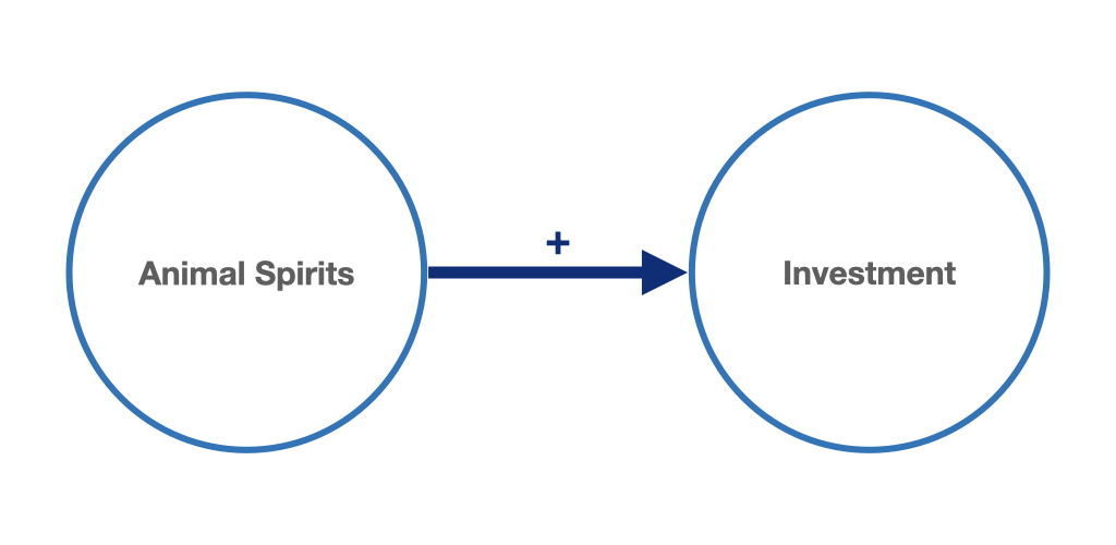
Figure 4.3: Animal Spirits have a positive effect on investment demand.
In the very general investment function shown with equation (4.1), we do not make any statements about the influence of other variables on investment demand. Nevertheless, we can make general statements about important factors affecting investment demand or animal spirits. For example, it seems plausible to assume that firms’ profit expectations play a central role in investment. If companies expect high capacity utilisation and full order books with good profitability, they will be willing to expand their production capacities or to invest in new technologies. Since companies’ expectations regarding actual future demand for their products are inherently uncertain, profit expectations may be subject to sudden fluctuations. Such changes in expectations could also affect the response of investment to other factors such as interest rates or capacity utilisation. In the case of fully exogenous investment demand, as in equation (4.1), a change in firms’ expectations would be represented by an exogenous (positive or negative) shock to animal spirits: \(\Delta I = \Delta a_a\). If we want to make a more accurate and systematic statement about how different exogenous or endogenous variables affect investment, we need to incorporate certain variables into our investment function. This will be done in the following subsections.
4.2 The effect of the interest rate on investment demand
The level of the expected real interest rate, \(r\), plays an important role in the investment decisions of firms (capital goods, equipment, commercial real estate) and households (residential real estate), since the real interest rate determines the financing costs of an investment and thus its profitability or even its feasibility. The real interest rate is given here by the nominal interest rate, \(i\), corrected for the expected inflation rate, \(\pi^e\). We obtain a simplified approximation of the real interest rate by:
\[\begin{equation} r = i - \pi^e \tag{4.2} \end{equation}\]
In the case of a loan-financed investment, the interest rate represents a direct cost factor of the investment project. If the investment is financed from the company’s own funds, e.g., from retained earnings, the company must weigh whether the real economic investment is more profitable than an alternative interest-bearing investment of the money.19 In investment theory, it is often assumed that the expected profitability of an investment can be calculated by the net present value of the investment. Here, the present value of the sum of the periodic cash surpluses expected from the investment, the so-called net present value, is compared with the acquisition cost of the investment itself.
\[\begin{equation} \text{Net present value} = \text{Present value of cash inflows} - \text{Acquisition cost} \tag{4.3} \end{equation}\]
From an economic point of view, if the net present value is positive, an investment is worthwhile. If it is negative, the investment involves a financial loss.
The periodic cash flow is the difference between the cash inflows and the cash outflows associated with the investment project in each period, excluding the initial expenditure on the investment project. Since the values of cash flows only occur in the future, we must use the interest calculation to make them comparable to the acquisition costs already incurred in the present. We obtain the present value of a future accruing cash flow by calculating how much we would have to invest today at a given interest rate to have a value of exactly that amount at the time of the potential cash flow. This value is called the present value.
The present value (\(V_t^e\)) of the cash flows expected in future time periods can thus be calculated as follows, where \(P_t^e\), \(P_{t+1}^e\), … to \(P_{t+T}^e\) stand for the expected cash flow in the time period \(t\), \(t+1\), etc. to \(t+T\), and for simplicity we assume that the real interest rate (\(r\)) remains constant over all periods:
\[\begin{equation} V_t^e = P_t^e+\frac{P_{t+1}^e}{\left(1+r\right)}+\frac{P_{t+2}^e}{\left(1+r\right)^2}+...+\frac{P_{t+T}^e}{\left(1+r\right)^T}\ =\sum_{i=0}^T\frac{1}{\left(1+r\right)^i}P_{t+i}^e \tag{4.4} \end{equation}\]
For a simple example, let us assume that the acquisition cost of a machine is €10,000 and that its use generates annual cash surpluses of €5200 over its life of two years. Assuming a real interest rate of 10%, the net present value of the investment would then be:
\[\begin{equation} \text{Net present value} = V_t^e - \text{Acquisition cost} \tag{4.5} \end{equation}\]
\[\text{Net present value} = 5200 € + \frac{5200 €}{1.10} - 10000 €\]
\[\text{Net present value}= - 72.73 €\]
The investment in this machine would therefore be loss-making at an interest rate of 10% and should not be carried out from an economic point of view. With a net present value of exactly 0, the project would be exactly on the threshold of profitability.
Since the present value of the cash flow depends on the assumed interest rate, the net present value also depends on the assumed interest rate. If we now calculate the theoretical interest rate at which an investment assumes a net present value of exactly zero, then we use it to calculate the interest rate at which the project is exactly at the threshold of profitability. Keynes called this interest rate the marginal efficiency of capital, or MEC for short.20 The MEC is also often referred to as the internal rate of return on the investment. If the interest rate charged to finance the investment exceeds the MEC of the project, the investment is loss-making and should not be undertaken by a profit oriented enterprise. However, if the interest rate is lower than the MEC, the investment is profitable. Keynes’s MEC is equal to the interest rate at which the present value of the cash flow is exactly equal to the cost of the investment:
\[\text{Acquisition costs} = \text{Present value of cash flows at MEC interest rate}\]
For the example from above we get:
\[10000€ = 5200 € + \frac{5200 €}{1 + \text{MEC}}\]
Rearranging for the MEC gives:
\[4800 € \cdot (1 + \text{MEC})= 5200 €\] \[4800 € \cdot \text{MEC}= 400 €\]
\[\text{MEC} = 0.083\]
Accordingly, the project would be profitable at an interest rate below 0.083%.
With such a simplified example, it should not be forgotten that the net present value and the MEC are very much characterised by uncertainty. The revenue and profit expectations of the companies can change quickly when new information about the business outlook emerges. This will then change the MEC accordingly, and at a given interest rate, more investment projects will be carried out at a higher MEC, or correspondingly fewer investments will be made at a lower MEC.
At a given point in time and with given revenue expectations, a number of investment projects are now possible in an economy. However, these projects will have different MEC. If we order these projects according to their MEC, and assume that the projects with the highest MEC are realised first, we obtain a falling curve of MEC as investment increases. This is shown in figure 4.4. Companies will now realise only those projects for which the MEC is higher than the interest rate on the credit market. As mentioned above, there are two main reasons for this. If the investments have to be financed at least in part by loans, servicing the loans requires that the companies generate corresponding revenues, i.e. the MEC is higher than the interest rate on the loan. If companies have sufficient internal funds and therefore do not dependent on loans, they will only invest even if the MEC exceeds the interest rate on the credit market. If this were not the case, they could alternatively lend their own funds at the prevailing interest rate on the credit market. From these considerations, we can therefore conclude that in the short run - and without considering further interactions in the model - there is a negative relationship between the realised investment volume and the level of the real lending rate at any point in time.
Figure 4.4: Marginal efficiency of capital, interest rate and investment.
Under these conditions, therefore, a rising real interest rate will have a negative effect on investment demand while a falling real interest rate should have a positive effect. The causality is illustrated in figure 4.5.
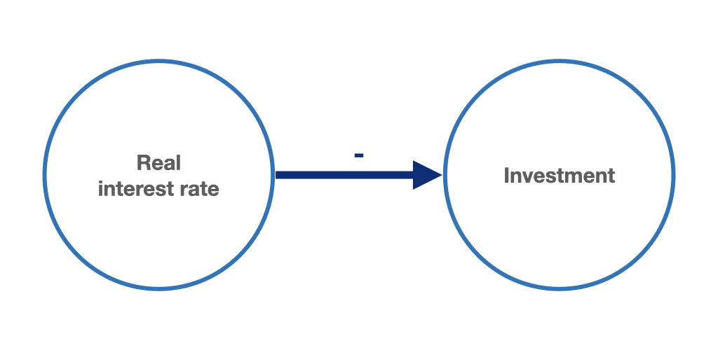
Figure 4.5: A higher real interest rate has a negative effect on investment demand.
The negative influence of the real interest rate is represented in the investment function by the term \(a_r r\). As mentioned above, however, there are other determinants of investment demand. In particular, the optimistic or pessimistic sales and revenue expectations of companies play an important role here. We therefore also take these into account in our investment function, since they are included in the animal spirits parameter, \(a_a\). A simple investment function that incorporates both the interest rate responsiveness of investment and other unspecified determinants of investment would therefore be:
\[\begin{equation} I = a_a - a_r r \tag{4.6} \end{equation}\]
The constant \(a_a\) is referred to here as autonomous investments or animal spirits. In addition, the real interest rate also has an impact, with the constant \(a_r\) being referred to as the interest rate sensitivity of investments. Here, it is assumed that a higher real interest rate has a negative impact on investments.
Lagged response of investment to the real interest rate
In addition to what was discussed above, we can assume that investments react to a change in the interest rate only with a certain delay (we then speak of a “lag” in the investment function).21 For example, it could be assumed that investments react to a change in the real interest rate only after a certain period of time, for example after one year. The investment function then becomes dynamic, i.e. investment in the current period, \(I\), is affected by the real interest rate of the previous period, \(r_{-1}\):
\[\begin{equation} I = a_a - a_r r_{-1} \tag{4.7} \end{equation}\]
Figure 4.6 represents the investment function from equation (4.7) for some hypothetical numerical values.
Figure 4.6: Investment function with animal spirits and interest rate sensitivity.
Together with Keynes’ investment theory, which is based on the marginal efficiency of capital, a negative influence of the interest rate on investment decisions can also be derived from the concept of the “principle of increasing risk” proposed by Michael Kalecki (1937). According to Kalecki, higher interest payments have a negative impact on investment because they burden companies’ retained earnings and reduce firms’ financial resources. Own financial resources are important for firms because access to external funds may be limited in incomplete financial markets. The level of a company’s own financial resources is usually a criterion for its creditworthiness and solvency affecting the potential amount of external funds that the company can raise. Moreover, an outflow of internal funds increases the risk for the company to become illiquid. An increased risk of illiquidity would in turn reduce the willingness of the management to invest in new capital stock.
The following interactive application allows to change the parameters of the investment function from equation (4.6).
4.3 The effect of demand on investment
Suppose that companies in our economy are faced with rapidly increasing demand for their products. Companies would meet the increase in demand first by selling their inventories of finished products and then by increasing production. If sales remain high, companies will experience and increase in the utilisation of their production capacity and will therefore decide to invest in new machinery, equipment and infrastructure. It is natural for companies to invest in new productive capacity if they expect the demand for their products to be high relative to their current production capacity. For the economy as a whole, we can make the simplifying assumption that high aggregate demand or high GDP has a positive impact on investment, as illustrated by figure 4.7.
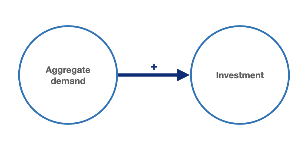
Figure 4.7: The accelerator effect: higher demand has a positive impact on investment.
In the investment functions presented so far, the revenue expectations improved with the increase in demand would be expressed by an improvement in the animal spirits represented by the constant \(a_a\). However, we can explicitly introduce the effect of demand into the investment function by inserting an additional term representing aggregate demand or aggregate income:
\[\begin{equation} I = a_a + a_Y Y - a_r r_{-1} \tag{4.8} \end{equation}\]
Here \(a_Y\) indicates the effect of demand on investment and it has a positive sign. This effect is also called the accelerator effect. The constant \(a_a\) is again interpreted as animal spirits and now expresses the general investment climate, the willingness of companies to take risks, etc. Compared to figure 4.6, the investment function from equation (4.8) in figure 4.8 is shifted upward thanks to the accelerator effect.
Figure 4.8: Investment function with animal spirits, interest rate responsiveness and accelerator effect.
The app accessible via the link below allows to interactively change the values of the parameters of the investment function seen with equation (4.8).
Further reading on chapter 4
Textbooks:
- Hein (2023, chaps. 3–4)
- Carlin and Soskice (2015, chap. 1)
- Snowdon and Vane (2005, chap. 2)
- Bofinger (2019, chap. 20) (in German)
- Heine and Herr (2013, chap. 4.3) (in German)
Other literature:
- Kalecki (1937)
- Keynes (1936, chaps. 11–12)
Literature
However, depending on the purpose of the model, the parameter \(a_a\) can also stand for the part of the investment that must be made in any case in order to remain competitive because of technological progress.↩︎
The interest rate would thus be a determinant of the opportunity cost which measures the lost profits from the financial investment of the money, in the case of equity financing of the investment.↩︎
This term is somewhat misleading, since it deals only with the marginal efficiency of the investment, and not with the entire capital stock. The term should therefore not be confused with the concept of marginal productivity of capital.↩︎
Lag means delay.↩︎