Chapter 6 The goods market equilibrium and the multiplier
In this chapter, we will develop a simple macroeconomic model of the demand side. To do this, we will need two main ingredients: an equilibrium condition and one or more behavioural equations. The purpose of this model is to illustrate the short-run processes of matching the supply of goods to the demand for goods. The equilibrium condition is satisfied when the demand for goods (\(Y_N\)) and the supply of goods (\(Y\)) are exactly equal and no more adjustment is needed. In other words, supply and demand have reached an equilibrium. We can summarize the equilibrium condition in the goods market with the following expression:
\[\begin{equation} Y_N = Y \tag{6.1} \end{equation}\]
This equilibrium condition is shown graphically in figure 6.1. The orange line is often referred to as the 45° line because it forms an angle of exactly 45° with both axes (when the axes are equally spaced). Along this line, the value of aggregate supply on the horizontal axis is exactly equal to the value of aggregate demand on the vertical axis. When the economy is on this line, the goods market of our economy is in equilibrium. In this situation, the plans of producers and the plan of consumers coincide so that in the goods market there is neither excess demand nor excess supply.
Figure 6.1: Goods market equilibrium.
When the economy is not in equilibrium (graphically not on the 45° line), an imbalance exists and a corresponding adjustment process is set in motion. How exactly this process takes place depends on the behavioural equations (which we still have to determine) of the different components of aggregate demand.
Since in this chapter we are only interested in the dynamics of aggregate demand, we assume that the supply of goods initially depends entirely on demand and that supply adjusts to changes in demand. We can say that the model is “demand driven”. This is a fundamental idea of Keynesian economic theory. For both post-Keynesian and new Keynesian economists, this approach is valid, at least in the short run. In the following sections, we will develop different variants of this short-run model, differing in particular in the number and in the complexity of the behavioural equations. We will draw on the behavioural equations of the individual components of aggregate demand elaborated in chapters 3 to 5. For the simplest version of the model, it is sufficient if we use the simple Keynesian consumption function from chapter 3) and consider the remaining components of aggregate demand as exogenous.
Figure 6.2: Demand-driven economy in the short run: the supply of goods adjusts to the demand for goods.
6.1 The simple income-expenditure model of a closed economy
In chapter 2, we have seen that aggregate demand in a closed economy is given by the sum of consumption demand, investment demand, and final government demand for goods and services. This can be summarised with the following formula \(Y_N = C + I + G\) where all variables are expressed in real terms, i.e., in constant prices. As described above, the goods market of an economy is in equilibrium when demand is equal to supply and production, which is to say that, in equilibrium, planned real expenditure, i.e. aggregate demand, \(Y_N\), is exactly equal to real aggregate output, \(Y\). Aggregate output \(Y\) represents also aggregate income, since the costs and profits incurred in production are also the income of producers to be divided between wages and profits. In equilibrium, we can use the terms expenditure, production and income as synonymous. Again, in equilibrium, they are also identical to gross domestic product (GDP). The goods market of the closed economy is therefore in equilibrium if the following condition is met:
\[\begin{equation} Y_N = C + I + G = Y \tag{6.2} \end{equation}\]
We can now insert into the equilibrium condition our behavioural equations for the individual components of demand from chapters 3 to 5. For the simplest version of our demand model, we initially consider only the simple Keynesian consumption function (equation (3.1) from chapter 3):
\[C = c_a + c_Y Y\]
Consumption is given by the sum of constant autonomous consumption, \(c_a\), and income-dependent consumption, \(c_Y Y\). The marginal propensity to consume, \(c_Y\), ranges from 0 to 1, \(0 < c_Y < 1\). For investment and government spending, we initially assume that they are fully exogenous.22 The behavioural equation of private consumption and the exogenous values for investment, \(\overline{I}\), and government spending, \(\overline{G}\), can now be inserted into the aggregate demand equation (2.1) of our closed economy from chapter 2:
\[\begin{equation} Y_N = c_a + c_Y Y + \overline{I} + \overline{G} \tag{6.3} \end{equation}\]
We can now represent graphically our aggregate demand function. To do so, we choose the following parameter constellation: for autonomous consumption: \(c_a = 30\), for the marginal propensity to consume: \(c_Y = 0.5\), for investment: \(\overline{I} = 10\) and for government spending: \(\overline{G} = 20\). In numbers, our demand function becomes:
\[Y_N = 30 + 0.5 \cdot Y + 10 + 20\]
or
\[Y_N = 60 + 0.5 \cdot Y\]
The numerical version of our aggregate demand function is shown in figure 6.3.
Figure 6.3: The demand function.
Indeed, figure 6.3 should remind us of the representation of our consumption function seen in figure 3.3. The dependence of demand on income arises here only because the variable part of consumption, \(c_Y Y\), depends on income. The other components of demand (autonomous consumption, investment and government spending) are exogenous and only affect the constant of the demand function, graphically represented by the intersection (or intercept) with the vertical axis. The slope of the demand function, the marginal effect of income on demand, is determined only by the marginal propensity to consume just as in the case of the simple Keynesian consumption function seen above.23
With the following interactive application, the values of the exogenous variables and parameters our simple aggregate demand function can be changed.
6.1.1 The equilibrium GDP
We now want to know the level of GDP at which the goods market of our economy is in equilibrium. In order to find this level, we need to calculate the level of GDP at which our equilibrium condition (\(Y_N = Y\)) is satisfied. We can derive the equilibrium level of GDP formally, i.e. using equations, but also graphically. Let’s start with the graphical derivation.
Graphical derivation
For the graphical derivation, we only need to merge the graphical representation of the equilibrium condition from figure 6.1 and the graphical representation of the demand function shown in figure 6.3. The result is reported in figure 6.4.
Figure 6.4: Goods market equilibrium in the income-expenditure model.
This figure represents the so-called income-expenditure model of the demand side of an economy. The income-expenditure model is often referred to as the “Keynesian cross”. The blue line is our demand function expressed as a function of income and the orange line is the equilibrium condition that we have defined above. The orange line also indicates the value of the supply of goods, since supply is equal to aggregate income (GDP). The equilibrium of our economy is given by the intersection of the two lines.
To the left of the equilibrium point, demand is higher than supply, so there is a surplus of demand. On the contrary, to the right of the equilibrium point, demand is less than supply and a supply surplus is recorded. If our economy is not in equilibrium, being either to the left or to the right of the 45° line looking at the figure 6.4, how does it move towards equilibrium?
This is done by an adjustment process leading to the so-called “multiplier effect”. We will describe first the formal derivation of equilibrium and then we will describe the adjustment towards equilibrium and the multiplier effect.
Formal derivation
In addition to the graphical derivation seen above, we can formally derive equilibrium GDP using the behavioural equations and the equilibrium condition of our model. To do this, we need to plug the behavioural equations into the equilibrium condition and solve for the endogenous variable, income or GDP.
We substitute into the equilibrium condition from (6.1), \(Y_N = Y\), that is, our demand function from equation (6.4), \(Y_N = c_a + c_Y Y^* + \overline{I} + \overline{G}\). However, to make it clear that this equation holds only in goods market equilibrium, we have added a small asterisk to the equilibrium income or GDP, \(Y^*\).
\[\begin{equation} Y^* = c_a + c_Y Y^* + \overline{I} + \overline{G} \tag{6.4} \end{equation}\]
We can now rearrange this equation step by step according to the equilibrium GDP, \(Y^*\), so we subtract \(c_Y Y^*\) on both sides of the equation:
\[Y^* - c_Y Y^* = c_a + \overline{I} + \overline{G}\]
and then collect \(Y^*\) on the left-hand side:
\[Y^* \left(1 - c_Y\right) = c_a + \overline{I} + \overline{G}\]
to finally divide both sides by \((1 - c_Y)\):
\[\begin{equation} Y^* = \frac{1}{\left(1 - c_Y \right)} \left( c_a + \overline{I} + \overline{G} \right) \tag{6.5} \end{equation}\]
We finally have an equation for GDP which represent the economy when is in equilibrium. But how does exactly the adjustment towards equilibrium work when the economy is out of equilibrium?
6.1.2 The adjustment process to the equilibrium and the multiplier
As we mentioned above, our short run model of the goods market is “demand-driven”, i.e. the supply on the goods market adjusts to the demand on the goods market. How does this happen?
Let us suppose that we are in a situation where demand is initially higher than supply. Let us also assume, as in figure 6.4, that the economy is initially in goods market equilibrium and that the demand curve shifts upward after an exogenous demand factor not related to income increases. Firms will respond to the excess demand by expanding output so that supply rises to its initial value on the new demand curve.
However, the expansion of production also means that the income of the economy increases because more workers receiving wages have to be hired for the higher production and because company owners record increasing profits thanks to higher sales. But since demand also depends on aggregate income (because of income-dependent consumption), the positive change in income will prompt demand to rise above its initial value. This means that the adjustment of supply to the initial surplus in demand has in turn led to a further surplus in demand! So firms will again adjust their production to meet demand by producing even more. This in turn leads to higher income, which in turn leads to higher demand, and so on.
So does this adjustment process never stop?
Of course not!24 We observe that although consumption increases as income increases, the increase in consumption is smaller than the increase in income. We obtain this by assuming the value of the marginal propensity to consume being between \(0\) and \(1\): \(0< c_Y < 1\). This means that in the second round of adjustment, firms’ output expansion is also lower than in the first round. Thus, demand and supply expansion become smaller and smaller during the adjustment process until supply finally “catches up” with demand. Then, demand for goods and supply of goods coincide again and the economy is back in equilibrium.
Figure 6.5: The multiplier effect in the case of initial excess demand (click play to start the adjustment process).
The adjustment process illustrated in figure 6.5 runs in detail as follows:
We are initially to the left of equilibrium in figure 6.5 at a demand, \(Y_N\), of 80 and a supply, \(Y\), of 40 (round 1 of the play slider).
That is, we have an initial excess demand (\(Y_N - Y\)) of 40, so firms will expand supply by 40, \(\Delta Y = 40\), to meet the higher demand (round 2 of the play slider).
However, the accompanying increase in wages and profits, and thus income, \(Y\), to 80 is reflected again in an increase in demand by 20 to 100 (\(\Delta Y_N = c_Y \cdot \Delta Y = 0.5 \cdot 40 = 20\)), as the economy’s income-dependent consumption demand increases (round 3). Thus, the new demand surplus here is 20, which is smaller than the initial demand surplus.
Firms will in turn meet this surplus demand and expand production and thus supply by 20 (round 4). Since the expansion of production is brought about by an increase in employment, wages and profits, and thus the income of the economy, will again increase by 20.
However, this again leads to an increase in income-dependent consumer demand. However, this renewed increase in demand is somewhat smaller than the previous one because the marginal propensity to consume is \(0.5\). Firms will increase production and thus employment again, so that income will rise again.
etc. … The resulting adjustment process and the underlying causality are illustrated in figure 6.6 and 6.7.
The adjustment process finally ends when supply is back at the same level as demand. The economy is back in equilibrium (\(Y^*\)).
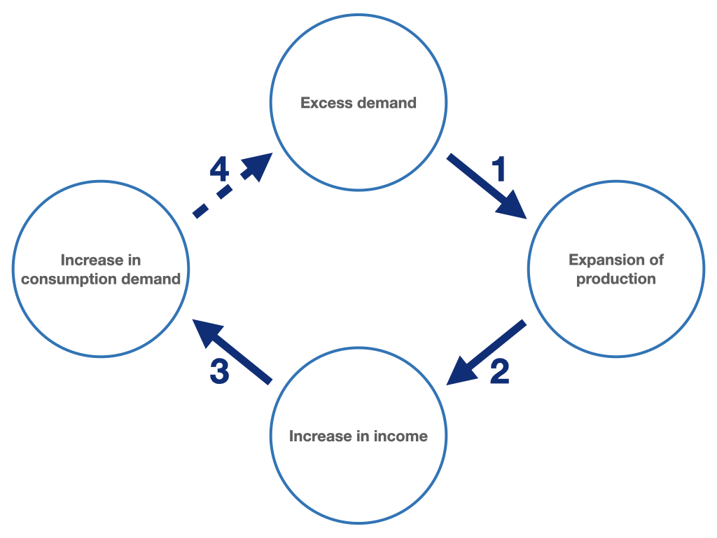
Figure 6.6: Conceptual representation of the adjustment process.
Figure 6.7: The multiplier effect in the case of initial excess demand: Adjustment after a demand shock.
The remarkable effect of the adjustment process shown in figures 6.5, 6.6 and 6.7 is that the increase in demand at the end of the adjustment is many times higher than the excess demand in the initial situation. Equilibrium output has thus been increased or “multiplied”, by a multiple of the excess demand as a result of the adjustment process. This effect is known as the “multiplier effect” and is an extremely important element of macroeconomic considerations and economic policy discussions.
In figures 6.5 and 6.7, the value of demand in the baseline situation is 80, while the GDP (i.e., income and output) of the economy is 40. However, GDP increases to a final value of 120 as a result of the adjustment to equilibrium. The initial demand surplus of 40 has resulted in a total increase (initial surplus + adjustment) in demand of 80 units (80/40 = 2). So the initial demand surplus have been multiplied by a factor \(\mu\) = 2. But how is this factor (the multiplier) determined?
We can derive the multiplier from equation (6.5) as follows, by deriving equilibrium income according to one of the autonomous expenditure components:25
\[\begin{equation} \mu = \frac{dY^{*}}{dI} = \frac{dY^{*}}{dc_a} = \frac{dY^{*}}{dG} = \frac{1}{1-c_Y} \tag{6.6} \end{equation}\]
In our simple model, the multiplier is determined solely by the marginal propensity to consume (\(MPC\)), \(c_Y\). Substituting the value of the \(MPC\) we determined above of \(c_Y = 0.5\) into equation (6.6) yields a value of 2 for the multiplier, exactly the value we had already calculated above. It is also evident from equation (6.6) that the multiplier becomes larger as the \(MPC\) increases (figure 6.8). For example, the multiplier would increase to 5 for an \(MPC\) of \(0.8\). Conversely, if the \(MPC\) falls, the multiplier decreases. At an \(MPC\) of \(0.2\), the multiplier would be only 1.25.
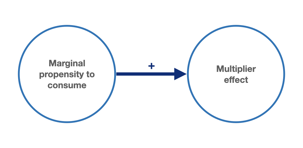
Figure 6.8: The higher the households’ marginal propensity to consume, the larger the multiplier.
6.2 Taxes in the income-expenditure model
6.2.1 Government expenditure multiplier with taxes independent of income
Now we want to introduce taxation into our model. In particular, we want to examine how the introduction of taxation affects the multiplier we derived in the previous paragraph. As we saw in section 3.2, we can start here by introducing taxation (\(T\)) as a lump sum independent of the level of income. Our consumption function becomes equation (3.7):
\[C = c_a + c_Y (Y - T)\]
Substituting this equation into the equilibrium condition (6.2) of the simple income-expenditure model, we obtain the following equilibrium value:
\[\begin{equation} Y^* = \frac{1}{(1 - c_Y)}(c_a - c_Y T + \overline{I} + \overline{G}) \tag{6.7} \end{equation}\]
In this case, the government expenditure multiplier \(\mu\) has not changed from equation (6.18). Only the expression \(- c_Y T\) has been added in parentheses in (6.7). We can now derive the tax multiplier \(\mu_T = \frac{dY^*}{dT}\), i.e., we can see how the equilibrium income \(Y^*\) changes when the government changes taxes:
\[\begin{equation} \mu_T = - \frac{c_Y}{(1 - c_Y)} \tag{6.8} \end{equation}\]
An increase in taxes (\(\Delta T>0\)) has a negative effect on equilibrium income, while a decrease in taxes (\(\Delta T<0\)) has the opposite effect. We can also observe that the absolute value of the tax multiplier is lower than that of the public expenditure multiplier. If, with a marginal propensity to consume of \(0.5\), we increase public spending by 1 million (\(\Delta G = 1\)), we obtain an increase in equilibrium income of 2 million. Conversely, if the government decides to stimulate the economy by cutting taxes by 1 million (\(\Delta T = - 1\)), national income increases by only 1 million.
Now assume that the government must avoid budget deficits and that government spending (\(G\)) is fully financed by tax revenues (\(T\)). We have that \(G = T\). What is the impact of an increase in government spending on equilibrium income? We now insert the balanced government budget condition (\(G = T\)) into the equilibrium income equation:
\[\begin{equation} Y^* = \frac{1}{(1 - c_Y)} \Big(c_a + \overline{I} + \overline{G} - c_Y \overline{G}\Big) \tag{6.9} \end{equation}\]
From this we get:
\[\begin{equation} Y^* = \frac{1}{(1 - c_Y)}\left(c_a + \overline{I} + \left(1 - c_Y \right)\overline{G} \right) \tag{6.10} \end{equation}\]
We obtain the multiplier for tax-financed public spending, \(\mu_{H_{G = T}}\), again by derivation with respect to \(G\):
\[\begin{equation} \mu_{H_{G = T}} = \frac{(1 - c_Y)}{(1 - c_Y)} = 1 \tag{6.11} \end{equation}\]
A budget-neutral spending policy has a positive impact on equilibrium GDP that is as large as the tax-financed spending increase itself: The multiplier (\(\mu_H\)) is equal to one when \(G = T\). This result is known as the Haavelmo theorem after the Norwegian economist Trygve Haavelmo (1945). How can the expansionary effect of tax-financed government spending be explained? By taxing, the government withdraws income from the household sector that would only be partially spent, because the marginal propensity to consume is less than one. The government, on the other hand, spends all of the tax revenue assuming \(G = T\). This then gives us the expansionary effect on equilibrium income.
6.2.2 Government spending multiplier with taxes based on income
In section 3.2, we had introduced taxation into the consumption function in a second step as a constant part of income, \(t Y\), where the net tax rate is \(0 < t < 1\). We can now combine the two tax categories and obtain a tax function composed of a fixed and an income-dependent part:
\[\begin{equation} T = T_a + tY \tag{6.12} \end{equation}\]
The value of equilibrium income thus becomes:
\[\begin{equation} Y^* = \frac{1}{\big(1 - c_{Y_d}(1 - t)\big)}\Big(c_a - c_{Y_d} T_a + \overline{I} + \overline{G} \Big) \tag{6.13} \end{equation}\]
We obtain the following multiplier for a change in taxation independent of income, \(T_a\):
\[\begin{equation} \mu_{T_a} = - \frac{c_{Y_d}}{\big(1 - c_{Y_d}(1 - t)\big)} \tag{6.14} \end{equation}\]
We have already seen in section 3.2 that the introduction of income-based taxation reduces the slope of the consumption function with respect to aggregate income (\(\frac{dC}{dY} = c_Y = c_{Y_d} (1-t)\)) because part of the income is withdrawn by the government. In this case, the Haavelmo multiplier will take a value smaller than 1:
\[\begin{equation} \mu_{H_{G = T_a}} = \frac{1 - c_{Y_d}}{\big(1 - c_{Y_d}(1 - t)\big)} < 1 \tag{6.15} \end{equation}\]
Suppose \(c = 0.5\) and \(t = 0.1\). If the government increases spending (\(\Delta G\)) by 5 million and fully finances this additional spending by increasing non-income taxes (\(\Delta T_a\)), equilibrium income increases by about 4.54 million, less than the fiscal stimulus of 5 million.
We can now once again summarise the entire income-expenditure model with taxes depending on income. The model now consists of the following equations.
- Aggregate demand (2.1): \[Y_N = C + I + G\]
- Consumption function (3.7): \[C = c_a + c_{Y_d} (Y - T)\]
- Tax function (6.12): \[T = T_a + tY \]
- Investment function (4.1): \[I = \overline{I}\]
- Government spending (5.1): \[G = \overline{G}\]
- Equilibrium condition (6.1): \[Y_N = Y\]
The graphical representation of the equilibrium in figure 6.9 differs from the previous one in figure 6.4 only in that in figure 6.9 both the slope and the intercept of the demand curve are smaller. This is due to the introduction of the tax function (6.12). As we have already learned, taxes as a constant fraction of income reduce the marginal propensity to consume from aggregate income and thereby reduce the slope of the demand curve. The non-income part of the slope function reduces the independent part of aggregate demand and thereby the intersection of the curve with the vertical axis.
Figure 6.9: Goods market equilibrium in the income-expenditure model with taxes depending on income.
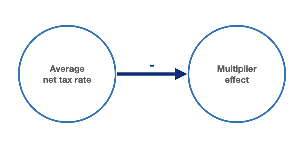
Figure 6.10: Higher net taxation of household income reduces the expenditure multiplier.
6.3 Employment and fiscal policy in the income-expenditure model
We have already mentioned a key concept several times in passing throughout our previous discussion of the adjustment process: the labour demand of firms in our simple Keynesian model economy depends on the demand for goods. For a given labour force (i.e., persons either already employed or seeking employment), unemployment or employment is determined by the demand for goods. We can now illustrate this relationship between aggregate demand and employment in our model.
For this purpose, we assume in a simplified way that exactly one worker is needed to produce one unit of goods. Thus, we establish a simple relationship between production, \(Y\), and the demand for labour, \(L\). We can call this relationship a simple production function. In this example, the production function is simply given by \(Y = L \frac{Y}{L}\), where \(\frac{Y}{L}\) is called labour productivity, which indicates how many units of output are produced per unit of labour (hour, day, week, or year). If \(\frac{Y}{L} = 1\), that is, if one worker produces exactly one unit of output per unit of time, then:26
\[\begin{equation} Y = L \tag{6.16} \end{equation}\]
The figure 6.11 combines our goods market equilibrium (the income-expenditure model) with the employment needed to produce GDP, with the goods market equilibrium on the left and the production function with the corresponding employment level on the right:
Figure 6.11: Goods market equilibrium with equilibrium employment.
The key insight here is that a change in aggregate demand will have employment effects in our model; a central proposition of Keynesian theory. If demand for goods increases, employment will rise and unemployment will fall; if, on the other hand, demand for goods falls, employment will fall and unemployment will rise.
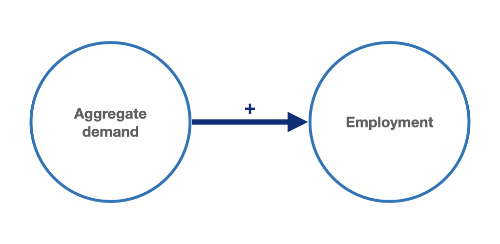
Figure 6.12: Given the relationship between production and labour input, demand for goods determines employment.
If we assume that the number of people willing to work in our example is 160, then the unemployment rate in equilibrium is 25% because only 120 of the 160 willing to work can actually be employed \((\text{unemployment rate} = ( 160 - 120 ) /160 \cdot 100 = 25 \%)\). In our simple model, therefore, policymakers can influence demand, and hence employment and unemployment, through government spending, \(\overline{G}\), assuming here that the government can also engage in credit-financed government spending (though we abstract from interest payments). The government’s use of government spending and government revenue is called fiscal policy. In our example, an economic policy that declares full employment as its goal should therefore adopt fiscal policy measures to solve the unemployment problem. The government would have to use “expansionary” fiscal policy which is to increase spending or cut taxes. In this context, the multiplier is of particular interest to economic policymakers as it determines how strongly demand, output and employment respond to a change in government spending and taxation. As we mentioned above, the absolute value of the government spending multiplier is larger than that of the tax multiplier in this context.
In the interactive app accessible through the link below, the role of the government can be assumed. The goal is to achieve full employment. Can full employment be produced by changing government spending and taxation? What is the effect of changing the multiplier on the fiscal policy needed to achieve full employment? The higher the other components of aggregate demand, the less the government needs to stimulate the economy to achieve full employment.27
Reality is much more complex than this simple income-expenditure model. It is far more difficult for policymakers to pursue successful economic policies, given also that economic policies have other goals and objectives besides full employment. Moreover, the so-called “fiscal space”, i.e. the government’s ability to increase government spending or cut taxes, may be limited or not used for other reasons. As the book progresses, we will identify other economic policy objectives and develop more complex models. However, our simple model nicely shows that demand, and therefore fiscal policy, has an effect on employment. This means not only that the government can reduce unemployment but also that the unemployment rate increases if the government cuts spending without stabilising (labour) demand through other measures or effects. Accordingly, a government demand shortfall can quickly lead to an increase in unemployment. The role of the state in managing labour demand was particularly evident during the financial and economic crisis of 2008/09 and the following euro crisis. In response to the financial crisis, many countries had initially pursued expansionary fiscal policies to mitigate the rise in unemployment caused by the drop in aggregate demand. In the following years, however, some countries switched to fiscal austerity, meaning spending cuts and higher taxes. This led to an increase in unemployment in many countries, as the loss of demand from the state caused by austerity measures was not sufficiently compensated by other demand components (cf. Hein 2013).
6.4 Interest rate sensitivity of investment in the income-expenditure model
Until now, we have assumed a very basic demand function for our simple income-expenditure model in which the only endogenous variables were private consumption and taxes. We have assumed government spending and investment to be completely exogenous. In this section, we will now develop an extended, but still very simple, demand model. The only change from the model of the previous subsection will be the assumption of an investment function in which investment depends on the real interest rate. Here, the real interest rate is assumed to be an exogenous variable, largely determined by the central bank’s interest rate policy and possibly by the situation on the credit market, which we will not discuss.28 We continue to regard government spending (\(\overline{G}\)) as exogenous and, for sake of simplicity, we also abstract from taxation.
In chapter 4 we saw that the real interest rate (\(r\)) can affect investment demand.29 With this change, investment will respond to changes in the interest rate. We set up an investment function consisting of a constant term, \(a_a\) (autonomous investment or “animal spirits”), and an interest rate sensitive term, \(-a_r r\), where \(a_r\) indicates the interest rate sensitivity of the investment. The negative sign in front of the second term means that investment demand decreases as interest rates increase. The investment function becomes:
\[\begin{equation} I = a_a - a_r r, \tag{4.6} \end{equation}\]
where \(a_r > 0\).
Our income-expenditure model with sensitivity of investment to the interest rate now consists of the following equations and its graphical representation is shown in figure 6.13:
- Aggregate demand (2.1): \[Y_N = C + I + G\]
- Consumption function (3.1): \[C = c_a + c_Y Y\]
- Investment function (4.6): \[I = a_a - a_r r\]
- Real interest rate: \[r = \overline{r}\]
- Government spending (5.1): \[G = \overline{G}\]
- Employment (6.16): \[L = Y\]
- Equilibrium condition (6.1): \[Y_N = Y\]
Figure 6.13: The demand function with interest rate sensitivity of investments.
Substituting equations (3.1), (4.6), (5.1) and the exogenous interest rate into equation (2.1), we obtain the demand function:
\[\begin{equation} Y_N = c_a + c_Y Y + a_a - a_r r + \overline{G} \tag{6.17} \end{equation}\]
Using the equilibrium condition (6.1) for the goods market, we can now again formally and graphically derive equilibrium GDP, \(Y^*\).
Formal derivation
The demand function (6.17) is substituted into the equilibrium condition (6.1) (\(Y_N = Y = Y^*\)):
\[Y^* = c_a + c_Y Y^* + a_a - a_r r + \overline{G}\]
\(c_Y Y^*\) is subtracted from both sides of the equation:
\[Y^* - c_Y Y^* = c_a + a_a - a_r r + \overline{G}\]
and then \(Y^*\) is collected on the left-hand side:
\[Y^* \left(1 - c_Y\right) = c_a + a_a - a_r r + \overline{G}\]
and finally, both sides are divided by \((1 - c_Y)\):
\[\begin{equation} Y^* = \frac{1}{\left(1 - c_Y \right)} \left( c_a + a_a - a_r r + \overline{G} \right) \tag{6.18} \end{equation}\]
With (6.18) we again have an equation for the GDP (or output or income) that occurs in goods market equilibrium. The multiplier, \(\mu = \frac{1}{\left(1 - c_Y \right)}\), is again included and, as much as before, defines equilibrium GDP as a multiple of the non-income demand components. The exogenous components are autonomous consumption, \(c_a\), autonomous and interest rate dependent investment, \(a_a - a_r r\) and government spending, \(\overline{G}\). The difference between the extended income-expenditure model and the simple model presented in the previous subsection is that the interest rate has now a negative effect on equilibrium aggregate demand due of its influence on investment.
Graphical derivation
The graphical derivation of the equilibrium does not differ from the derivation in the previous subsection. The representation of the two functions in a diagram with demand on the vertical axis and income on the horizontal axis is unchanged. However, the content of the two functions differs because the interest rate now exerts an effect on aggregate demand and it has an impact on equilibrium as shown in figure 6.15. This in turn means that employment also depends on the interest rate.
For the graphical derivation, we revert to our numerical example of the simple model that we have seen previously. The goods market equilibrium and equilibrium employment are shown in figure 6.14. In purely visual terms, the figure is no different from figure 6.11. However, an increase in the real interest rate would now shift the demand function downward in parallel, leading to lower equilibrium income and employment.
Figure 6.14: Goods market equilibrium and equilibrium employment with interest rate sensitivity of investment.
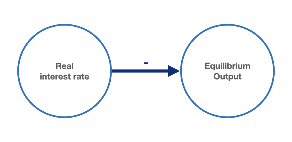
Figure 6.15: A higher real interest rate has a negative impact on the macroeconomic equilibrium.
In chapter 7, we will revisit the relationship between interest rates and macroeconomic equilibrium and discuss how the central bank’s interest rate policy can affect the performance of the overall economy.
6.5 Accelerator effect in the income-expenditure model
In this final section, we extend the model that we have being developing above. We will include an additional component in the investment function that makes investment also dependent on aggregate demand, just as we learned in section 4.3. A positive effect of aggregate demand on investment seems a plausible assumption. When aggregate demand increases, firms have to increase their productive capacity in order to meet the rise in demand. The demand-induced marginal increase in investment, also called the accelerator effect, \(a_Y\), acts in our goods market model similarly to the income-induced marginal increase in consumption demand, \(c_Y\). An initial stimulus in aggregate demand (“a demand shock”) leads in turn to an increase in demand via the accelerator effect and the marginal propensity to consume. Both elements have a positive impact on the multiplier. Our goods market model with the additional accelerator effect is now given by the following set of equations:
- Aggregate demand (2.1): \[Y_N = C + I + G\]
- Consumption function (3.1): \[C = c_a + c_Y Y\]
- Investment function (4.8): \[I = a_a - a_r r + a_Y Y\]
- Real interest rate: \[r = \overline{r}\]
- Government spending (5.1): \[G = \overline{G}\]
- Employment (6.16): \[L = Y\]
- Equilibrium condition (6.1): \[Y_N = Y\]
The only difference from the model seen in section 6.4 is the new version of the investment function (4.8) now incorporating the effect of aggregate demand.
Formal representation of the equilibrium
We can formally obtain the equilibrium just in the same way as we did above:
\[\begin{equation} Y^* = \frac{1}{\left(1 - c_Y - a_Y \right)} \left( c_a + a_a - a_r r + \overline{G} \right) \tag{6.19} \end{equation}\]
The multiplier has now become \(\mu = \frac{1}{\left(1 - c_Y - a_Y \right)}\) and its value is now higher. Assuming that \(c_Y = 0.5\) and \(a_Y = 0.1\), we get a value of the multiplier \(\mu\) = 2.5, clearly larger than the value of the multiplier without the accelerator effect. If the government increases spending (\(\Delta G\)) by 1 million, equilibrium income increases by 2.5 million.
Graphical representation of the equilibrium
The graphical representation of the equilibrium in figure 6.16 differs only with respect to the slope of the aggregate demand function. The introduction of the accelerator effect, \(a_Y\), leads to a steeper function and to a higher value of the multiplier.
Figure 6.16: Goods market equilibrium and equilibrium employment with an accelerator effect in the investment function.
To conclude, we can state that the income-expenditure model of the goods market that we discussed so far can always be reduced to the product of the multiplier, \(\mu\), and of the income autonomous demand, \(Y_{N_a}\).
\[\begin{equation} Y^* = \mu Y_{N_a} \tag{6.20} \end{equation}\]
We have also seen how the introduction of additional income or demand-dependent model components can change the size of the multiplier. The introduction of a tax function that depends in part endogenously on income levels has reduced the value of the multiplier. On the contrary, the introduction of a demand-dependent investment function (accelerator effect) has had a positive effect on the value of the multiplier. We have also learned how the introduction of exogenous variables (e.g., the real interest rate in the investment function) does not directly affect the value of the multiplier. However, the change in the value of an exogenous variable due to the effect of the multiplier always has a larger effect than the initial stimulus itself.
The interaction of the multiplier and income autonomous demand determine the goods market equilibrium (figure 6.17).
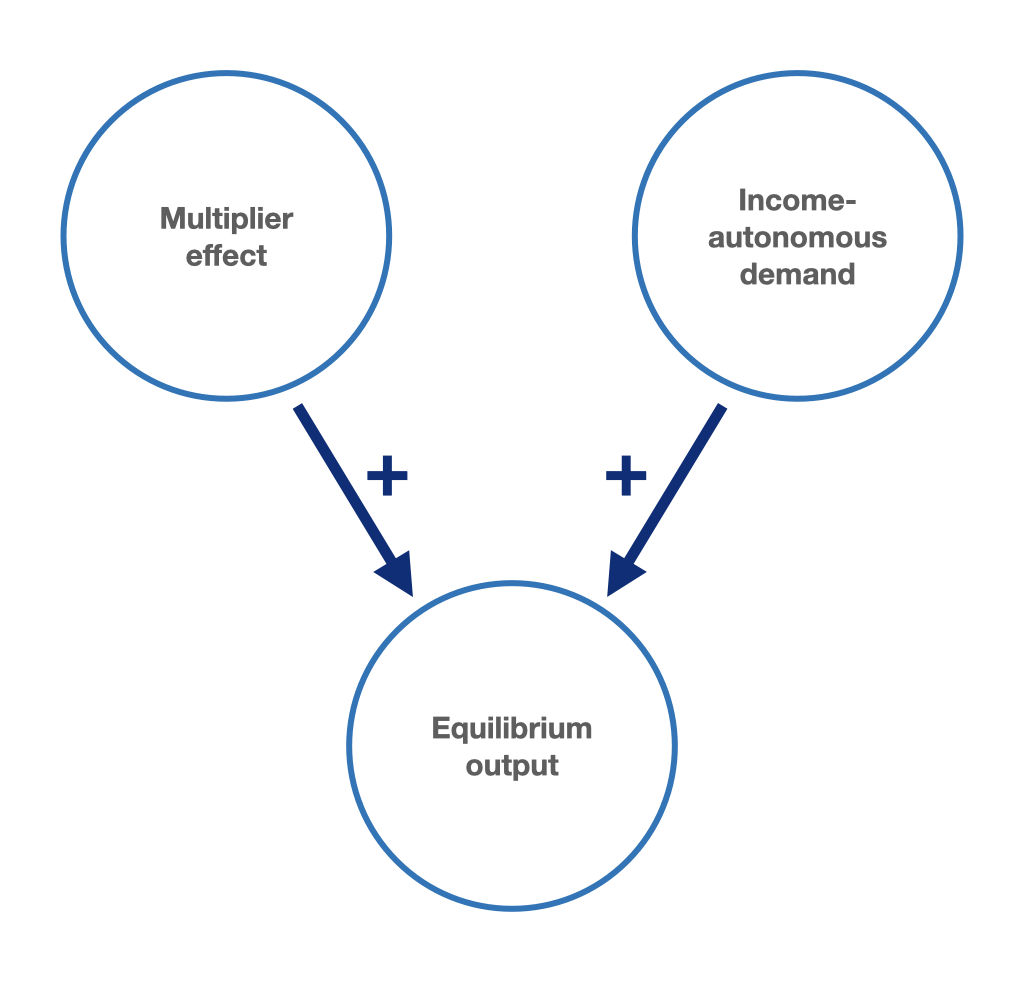
Figure 6.17: Multiplier and income autonomous demand determine the goods market equilibrium.
Further reading on chapter 6
Textbooks:
- Hein (2023, chap. 4)
- Carlin and Soskice (2015, chap. 1)
- Heine and Herr (2013, chap. 4.4) (in German)
- Heine and Herr (2013, chap. 6.4.1) (in German)
Other literature:
- Haavelmo (1945)
Literature
Endogenous variables are determined only by “solving” a model. Thus, they depend on other model variables and parameters. Exogenous variables are independent of other variables and parameters of the model. In other words, they are determined outside the model.↩︎
This would change if, for example, we were to include an accelerator effect in our investment function, as in equation (4.8).↩︎
At least the differences between supply and demand become infinitesimally small as the adjustment proceeds.↩︎
For an alternative derivation of the multiplier, see appendix G.↩︎
More on the relationship between employment and output in chapter 8.↩︎
In this example, labour productivity is fixed at a value of 1.↩︎
Compare e.g. Heine and Herr (2013, chap. 4.3).↩︎
In our income-expenditure model, the price level is constant, therefore there is no inflation and the real and nominal interest rate are equal (why?).↩︎