Chapter 9 Inflation - the conflict between wage and profit claims

A central aspect of economic policy discussions revolves around the rate of change of the average price level of an economy, the so-called inflation rate. A very rapidly and sharply changing price level is usually associated with destabilising effects. For example, high and rising inflation rates can cause the population to lose confidence in the currency and lead to a flight into real assets (or other currencies). Deflation, i.e. generally falling prices, can easily lead to or exacerbate a deep economic crisis, as consumption and investment spending are “postponed” and the real debt burdens of companies and households explode. Since nominal interest rates - and of course nominal interest payments on the loan - are agreed in loan contracts, debtors have to earn more and more in real terms when prices fall in order to meet their nominal payment obligations. Real debt thus increases and with it the likelihood that it can no longer be serviced, leading to widespread insolvencies and bankruptcies.

In this chapter we want to develop an understanding of how changes in the general price level occur, i.e. how inflation or deflation occurs. In general, we understand inflation as a process resulting from a bargaining conflict between firms and employees over the appropriate real wage. Inflation is therefore the result of a distributional conflict. To understand this, we will develop simple models of the real wage targets of firms and workers. At the heart of the emergence of inflation and deflation is the bargaining power of the respective actors. In the next section we start with the wage demands of employees.

9.1 Wage bargaining in the “labour market” and the real wage targets of employees

For our macroeconomic model and the relationship between inflation and wages, we need an aggregate model of wage bargaining in the “labour market”. However, wages are usually negotiated at the firm and industry level and in some cases even for whole sectors (e.g. the public sector), in some countries also for the economy as a whole. In the context of our macroeconomic model, we are interested in the overall effect of these negotiations on the average wage rate. We thus assume that individual bargaining, at whatever level, is aggregated.

The essential concept that explains the wage demands of employees in our model, both at the micro and macro level, is bargaining power. This bargaining power depends, on the one hand, on institutional conditions such as the degree of unionisation (union density), the degree of coverage of collective bargaining, the degree of coordination of unions and collective bargaining, the amount and duration of wage replacement benefits, and employment protection legislation. Fundamental changes in these areas usually only take place in the long term. Given institutional conditions, bargaining power is then influenced on the other hand by the level of employment or the unemployment rate, which can also change significantly in the short term. When employment is high or the unemployment rate is low, it tends to be easier for employees to find a job or to change jobs. The fear of not finding a job or even losing a job due to too high wage demands is significantly lower than in a situation of high unemployment. Companies, on the other hand, face high demand for their products when employment is high, and in order to produce them, they have to keep employment at a high level even if employees demand higher wages. The employees, or the institutions that represent them (trade unions), will accordingly be able to enforce higher nominal wage demands against the companies.

The nominal wage, \(w_{n}\), is accordingly a positive function of employment, \(L\), institutional factors and social norms, \(\mathbf{b}\) (union density, degree of coverage of collective bargaining, degree of coordination of unions and collective bargaining, level and duration of wage replacement benefits, employment protection legislation), and the expected price level, \(P^e\):

\[\begin{equation} w_{n} = f(L,\mathbf{b}, P^e) \tag{9.1} \end{equation}\]

While wage negotiations are conducted on nominal wages, the real objective of employees and trade unions is a certain real wage. The real wage, \(w_{r}\), measures the quantity of goods that can be bought at the current price level with the nominal wage. The real wage is therefore the nominal wage corrected for the price level, i.e. the ratio of the nominal wage rate, \(w_{n}\), and the average price level, \(P\):

\[\text{Real wage} = \frac{\text{Nominal wage €}}{\text{Price level €}}\] or

\[\begin{equation} w_{r}= \frac{w_{n}}{P} \tag{9.2} \end{equation}\]

We can now express the real wage target of employees, \(w^{ws}_{r}\), as the ratio of nominal wage demands to the expected price level:

\[\text{Real wage target of employees} = \frac{\text{Nominal wage claim €}}{\text{Expected price level €}}\]

\[\begin{equation} w^{ws}_{r} = \frac{w_{n}}{P^e} \tag{9.3} \end{equation}\]

For our model of wage demands we can now state that the higher the employment level, the higher the real wage, \(w^{ws}_{r}\), that the employees or the trade unions try to achieve through their nominal wage demands. In the case of a very low level of employment, however, we also assume that there is a minimum real wage which the trade unions want to enforce regardless of the level of employment. This minimum can be determined, for example, by social benefits and minimum wages as well as social norms.

We can now describe the relationship between the real wage target of the employees or trade unions and the employment level, \(L\), by the so-called wage-setting curve, or the target real wage rate curve, which is given by the following equation:³²

\[\begin{equation} w^{ws}_{r} = \mathbf{b} + k L, \quad \text{where} \quad \mathbf{b}, k > 0 \tag{9.4} \end{equation}\]

In equation (9.4), the various factors that determine the real wage minimum are summarised in the variable \(\mathbf{b}\), and the parameter \(k\) determines the slope of the wage-setting curve. The slope of the wage-setting curve describes the ability of employees and trade unions to exert pressure on companies in wage negotiations, e.g. in the form of strikes, a reduction in efficiency at the workplace or the rejection of a job offer. We can also interpret the slope of the curve as an expression of the conflict-orientation of the workers. Both the constant, \(\mathbf{b}\), and the slope, \(k\), of the wage-setting curve therefore depend on the institutional conditions of wage bargaining mentioned above. Figure 9.1 illustrates the wage-setting curve.

Figure 9.1: The wage-setting curve.

It shows a linear relationship between the real wage target and employment. The higher the employment level, the higher the real wage targets of employees. Thus, given inflation expectations, nominal wage demands will rise correspondingly with employment.

Figures 9.2 and 9.3 illustrate that employment, \(L\), can be seen as a cyclical factor of wage demands, while the institutional framework conditions and social norms of the labour market and thus of wage bargaining as structural factors have a rather long-term effect on the target real wage of employees via their effect on \(\mathbf{b}\) and \(k\).

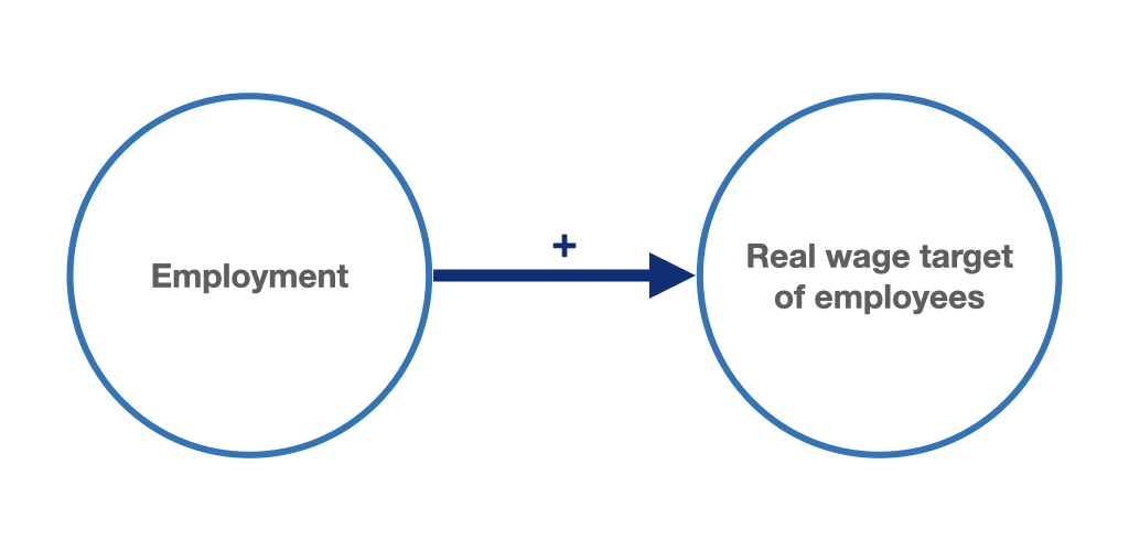
Figure 9.2: Cyclical target real wage: higher employment levels lead to higher wage demands.

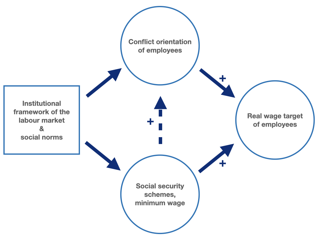
Figure 9.3: Institutional conditions and social norms determine the conflict orientation of employees and thus the target real wages.

9.2 Price-setting and the real wage targets of companies

So far, we have only talked about the target real wage rates of employees, which then determine their nominal wage demands. These determine the price of the factor labour, which enterprises have to include as a cost factor in their production plans and price determination. For the sake of simplicity, we assume in the following that employees can also enforce their nominal wage demands on the labour market and thus determine the nominal wage costs of enterprises. The crucial question for the emergence of inflation and deflation is now how nominal wages and the price level are related.

In our simplified production function, \(Y = y L\), from chapter 8, the variable production costs of firms are given by the product of labour input and nominal wages, thus consisting only of wage costs. We refrain here from considering other variable costs, such as costs for raw materials or semi-finished products. In addition to the variable wage costs, only fixed capital costs are incurred, i.e. depreciation on the capital stock and, if applicable, interest on borrowed capital. We will return to their explicit treatment below. Here we first treat these costs as part of enterprise profits. The following now applies to variable production costs:

\[\begin{equation} \text{Variable production costs} = \text{Wage costs} = \text{Nominal wages} \cdot\text{Employment} = w_{n}\cdot L \tag{9.5} \end{equation}\]

The labour costs per output produced, the so-called unit labour costs, result accordingly from the ratio of labour costs and total production, i.e. output, \(Y\):

\[\begin{equation} \text{Unit labour costs} = \frac{\text{Labour costs}}{\text{Output}} = \frac{w_{n} L}{Y} \tag{9.6} \end{equation}\]

If we now substitute our production function, \(Y = y L\), into this equation, we get:

\[\begin{equation} \text{Unit labour costs} = \frac{w_{n} L}{yL} = \frac{w_{n}}{y} \tag{9.7} \end{equation}\]

Since, according to our production function, labour productivity (up to full utilisation of the production capacity given by the capital stock, \(Y^p\)) is constant, firms also face constant unit labour costs at a constant nominal wage rate, as shown in figure 9.4. With a higher nominal wage rate, the unit labour cost curve would shift upwards in parallel accordingly.

Figure 9.4: Prices and production costs.

For our simple model of price formation, we now assume that firms set their prices on the basis of their average variable costs of production, i.e. unit labour costs.³³ Firms add a profit margin to these costs, the “mark-up”, for the profit per unit. This so-called mark-up pricing, which was introduced into macroeconomic theory by Michal Kalecki (1954, chap. 1; 1971, chap. 5), occurs above all in those goods markets in which, on the one hand, the companies have a certain pricing power and, on the other hand, with free production capacities, firms can react to increases in demand at short notice with increases in production and supply. In these oligopolistic or monopolistic markets, price competition is limited and firms act as quantity adjusters to changes in demand, as we have assumed throughout this book so far. Such markets are a typical feature of developed capitalist economies where, especially in the industrial sector, there are usually only a limited number of firms competing with each other. Take, for example, the markets for smartphones or computer chips, where only a few global players meet a large number of customers. But also in the service sector, for example in the area of search engines and e-commerce, there are often only a few companies that largely dominate the market.

Determinants of the mark-up

The level of mark-up is determined by various structural factors of the branches of production in the industrial and service sectors of the economy (see Hein 2014, chap. 5.2; Kalecki 1954, chap. 1; 1971, chap. 5). The mark-up depends positively on the degree of concentration in the respective branches of production, negatively on the importance of price competition relative to other forms of competition (marketing, product differentiation), and negatively on the structural strength of the trade unions, which is determined, among other things, by the above-mentioned structural factors of the labour market and social security systems. In addition, the mark-up must also cover costs other than unit labour costs, such as interest costs and other capital or overhead costs. If these costs change for all or the majority of enterprises in a production sector, a change in the mark-up can be expected in the same direction. However, all these determinants of the mark-up tend to have a long-term influence, so that in the following we will disregard them for the time being and assume a constant mark-up in the short term.

Thus, if we assume that imperfect competition and underutilised production capacities given by the capital stock are the normal case in our capitalist model economy, then mark-up pricing by firms leads to the following price equation:

\[\begin{equation} P= (1+m) \frac{w_{n}}{y} \tag{9.8} \end{equation}\]

The mark-up thus determines the gross profit per unit of output, which is then available to cover fixed capital costs and the various profits (interest, dividends, rents, leases, retained earnings).

From our price equation we can now also derive a real wage target for firms. The price-setting real wage, \(w^{ps}_{r}\), or the firms’ target real wage rate, is the real wage that coincides with the firms’ profit targets. To derive it, we solve the equation (9.8) for the real wage rate, \(w_r = w_n / P\), and this yields the price-setting curve, which is the firms’ target real wage rate.

\[\begin{equation} w^{ps}_{r} = \frac{w_n}{P} = \frac{y}{(1 + m)} \tag{9.9} \end{equation}\]

Thus, firms’ target real wage rate depends positively on labour productivity and negatively on mark-up (figures 9.5 and 9.6). The higher the labour productivity, the higher the real wage rate compatible with firms’ profit targets. The higher the mark-up, the lower the real wage rate compatible with the profit targets.

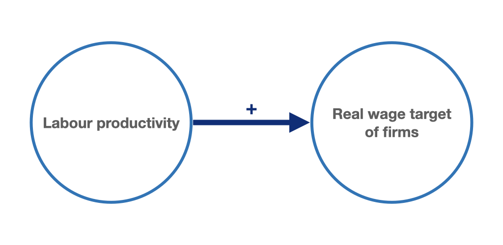
Figure 9.5: Higher labour productivity allows for higher real wages while companies’ profit margins remain the same.

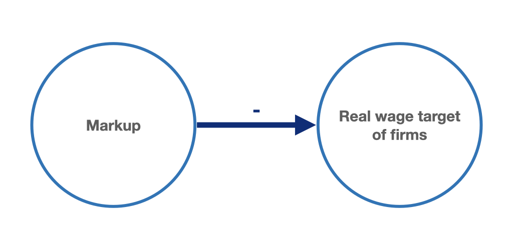
Figure 9.6: Higher mark-up leads to decreasing real wage target of enterprises.

For a given labour productivity and mark-up in the short run, the firms’ target real wage rate does not change with output and employment changes. The price-setting curve in figure 9.7 therefore becomes horizontal.

Figure 9.7: Price-setting curve.

9.3 Wage-setting, price-setting and equilibrium distribution

We can now use the wage-setting curve (\(WS\) curve), which represents the real wage targets of employees, and the price-setting curve (\(PS\) curve), which represents the real wage targets of firms, to show in figure 9.8 the equilibrium distribution in our model economy in which the target real wages of employees and firms coincide.

Figure 9.8: Wage-setting curve, price-setting curve and equilibrium distribution.

The intersection of the price and wage-setting curves determines the level of employment at which the real wage targets of employees coincide with the unit profit targets and thus the real wage targets of firms. This point is sometimes misleadingly interpreted as labour market equilibrium. Instead of an equilibrium on the labour market, it is a distributional equilibrium, which is derived from wage setting on the labour market in connection with price setting on the goods market. So there are two markets at play here, not just the labour market. employees and trade unions set the nominal wage rate on the labour market in order to achieve their real wage target. Companies set the price of goods on the goods market in order to achieve their profit target and thus implicitly their real wage target. Only when both actors achieve their goals do we have a distributional equilibrium. We will see below that only this equilibrium is then accompanied by constant inflation. Deviations from the equilibrium upwards or downwards then entail rising or falling inflation rates. We will also see that changes in employment determined by the distributional equilibrium do not yet mean that actual employment in the labour market changes. Therefore, equilibrium employment determined by the wage-setting and price-setting curves should in no case be called labour market equilibrium.

As figure 9.8 shows, this equilibrium is usually accompanied by involuntary unemployment and equilibrium employment is below the maximum possible full employment level for a given labour force. The equilibrium is therefore not an equilibrium in the sense of market clearing, but only refers to the agreement of the real wage targets of workers and companies. If the model economy is in this situation, both the expectations of the companies with regard to their profit margins and the expectations of the workers with regard to their real wages are fulfilled. For both groups, it follows that they do not need to change their behaviour further as long as employment does not deviate from this equilibrium.

We can also formally derive the distribution equilibrium. All we have to do is equate the equations for the wage and price-setting curves (9.10) and solve for the employment corresponding to the distributional equilibrium, \(L^N\) (9.11):

\[\begin{equation} \mathbf{b} + kL^N = \frac{y}{(1 + m)} \tag{9.10} \end{equation}\]

\[\begin{equation} L^N = \frac{1}{k}\left[\frac{y}{(1 + m)} - \mathbf{b}\right] \tag{9.11} \end{equation}\]

There is therefore only one level of employment, and with a given labour supply thus only one unemployment rate, at which the real wage targets, and thus the distribution targets, of employees and trade unions on the one hand and companies on the other hand coincide with each other and are therefore compatible with each other. We can therefore interpret this level of employment, and the corresponding unemployment rate, as an expression of a distributional equilibrium.

However, as we will see, this equilibrium is not necessarily stable, in the sense that there is no automatic return to distributional equilibrium in case of deviations. To understand this process, we must first examine the mechanism that can cause a change in the price level in the wage bargaining and price setting model just described.

An important difference: \(L^*\) vs. \(L^N\)

We must clearly distinguish between the actually realised employment level \(L^*\), which is conditioned by the equilibrium of the goods market, and the employment level \(L^N\), which is determined by the distribution equilibrium. \(L^*\) is determined by the actual demand on the goods market and changes whenever the determinants of aggregate demand change. \(L^N\) is not determined here by the effective demand, but initially only by the distribution claims of firms and employees. As a rule, \(L^*\) will deviate from \(L^N\), and we will analyse the consequences of such a deviation in the following.

9.4 The inflation rate as an expression of a distributional conflict: inflation-stable employment and the NAIRU

We have already said above that the objective of price setting is to secure the target profit margin of firms, i.e. the target profit per unit. However, this goal can only be achieved by firms if the real wage does not rise above the level of the price-setting curve, which after all indicates the implicit target real wage rate of firms. The distributional conflict between wages and profits and thus between labour and capital can be illustrated by the price-setting curve. Figure 9.9 shows the real wage target of firms (the \(PS\) curve) compared to output per labour input, i.e. labour productivity.

Figure 9.9: The corporate price-setting curve and the distributional conflict between capital and labour.

The upper horizontal line in the figure shows labour productivity, i.e. output per labour input. The income made possible by this is now divided between profits and wages. The part of the output that lies between the real wage curve and labour productivity goes to the enterprises as profits. In total, the enterprises receive the real profit sum: \(\Pi_r = y L - w_rL\). Everything below the real wage curve goes in the form of wages to the workers, who receive the total real wage sum \(W_r = w_r L\). The total area below the labour productivity line to the horizontal axis represents total economic production at full employment (Real Production: \(Y = y L\)). When employment and total output fall to lower levels, the sum of profits, \(\Pi_r\), and the sum of wages, \(W_r\), fall, but their ratio to total output, \(\Pi_r / Y\) and \(W_r / Y\), respectively, remains constant - at least as long as the price-setting curve in the figure does not shift. We can interpret this relationship as the functional distribution of income between capital and labour (see Hein 2014, chap. 1).

If we now add the wage-setting curve to the figure, it becomes clear that equilibrium employment is accompanied by a certain distribution of income, or better, equilibrium employment is determined by a distributional equilibrium in which the distributional goals of firms and workers coincide. We have assumed here that firms are always able to enforce their target real wage due to their pricing power.

Figure 9.10: The price-setting curve of enterprises, the wage-setting curve of workers and the distributional equilibrium.

In the following interactive application, the parameters of the figure 9.10 can be changed:

Link to the app

Figures 9.10 and the relative interactive application nicely illustrate that a distributional conflict underlies the wage and price-setting behaviour of the bargaining parties in our economy. But how is this conflict related to the inflation rate? We can understand this if we are clear about what happens in the model when the level of employment rises above the equilibrium value \(L^N\) and the workers try to impose a higher real wage. Such a situation can be caused, for example, by a positive demand shock. In this case we are therefore to the right of the equilibrium point \(L^N\). The wage and price-setting process in this case proceeds as follows:

Employment is at a level above equilibrium, e.g. as a result of the demand shock.
employees and trade unions demand stronger increases in nominal wages in order to realise a higher real wage, initially assuming that the price level grows at the previous rate of inflation.
Companies concede the nominal wage increase.
But immediately after the nominal wage increase is negotiated, the companies realise an impending fall in their profit margin.
In order to defend their profit margin, the companies raise prices, and thus the inflation rate, just enough to restore the original real wage.
Thus we observe an increase in the inflation rate. This results from a conflict between target real wages and profits, or between employees and enterprises, which the enterprises can temporarily decide in their favour through an increase in the inflation rate.
However, the employees have not reached their target and will therefore force the increase in nominal wages in the next period, which will then also cause the inflation rate to rise further.

The movement of the inflation rate as a function of employment, which is triggered by the behaviour just described, can be described with the concept of the Phillips curve, which describes the relationship between employment (or unemployment) and the inflation rate.

If employment is above \(L^N\), i.e. \(L > L^N\), employees will try to increase the real wage to their target real wage rate in accordance with the \(WS\) curve (equation (9.4)). Thus, the change in the real wage intended by the employees is given by the difference between the target real wage, \(w^{ws}_{r}(L)\), which depends on realised employment, and the actual realised real wage of the last period, \(w_{r,-1}\), i.e. as:

\[w^{ws}_{r}(L) - w_{r,-1}\]

However, since firms can always reset the real wage to their target wage by setting prices, the realised real wage of the last period is exactly the firms’ target real wage, \(w^{ps}_{r} = w_{r,-1}\). Here we assume, as explained above, that the firms’ target real wage is constant. We therefore do not need a time index for it that refers to the previous period (i.e. no \(_{-1}\)). The target real wage of firms coincides with the target real wage rate of employees only at the intersection of the \(PS\) and \(WS\) curves, i.e. only when the employment level is \(L^N\). It then holds:

\[L = L^N\]

\[w^{ps}_{r} = w^{ws}_r = \mathbf{b} + kL^N\]

Thus, for the change in the real wage intended by employees at \(L > L^N\), \(w^{ws}_{r}(L) - w_{r,-1}\), we can write the following:

\[\begin{equation} w^{ws}_{r}(L) - w_{r,-1} = w^{ws}_{r}(L) - w^{ps}_{r} = w^{ws}_{r}(L) - (\mathbf{b} + kL^N) \tag{9.12} \end{equation}\]

For \(w^{ws}_{r}(L)\) we can also simply substitute the equation (9.4) of the \(WS\) curve into equation (9.12):

\[w^{ws}_{r}(L) - w_{r,-1} = \mathbf{b} + kL - (\mathbf{b} + kL^N)\]

\[w^{ws}_{r}(L) - w_{r,-1} = kL - kL^N\]

By factoring out the parameter of the conflict orientation of the employees or trade unions, \(k\), we finally obtain:

\[\begin{equation} w^{ws}_{r}(L) - w_{r,-1} = k(L - L^N) \tag{9.13} \end{equation}\]

The change in the real wage intended by the employees is thus dependent on the conflict orientation and the gap between the employment level determined by the goods market equilibrium and that determined by the distribution equilibrium, \(L - L^N\).

However, since wage negotiations are conducted on the nominal wage, \(w_{n}\), the employees must enforce a certain nominal wage in the negotiations in order to achieve their real wage target. In doing so, employees must of course also take into account their expectations regarding the inflation rate, \(\pi = \Delta P/P_{-1}\), since the inflation rate ultimately changes the relationship between nominal wage and price, i.e. the real wage, \(w_{r} = w_{n}/P\). For the change in the real wage, therefore, both the change in the nominal wage and the inflation rate are important. The change in the real wage, \(w_{r} - w_{r,-1} = \frac{\Delta w_{r}}{w_{r, -1}}\), is approximated as the difference between the wage inflation rate, \(\Delta w_{n}/w_{n, -1}\), and the price inflation rate, \(\pi = \Delta P/P_{-1}\):

\[\begin{equation} w_{r} - w_{r,-1} \approx \frac{\Delta w_{n}}{w_{n, -1}} - \pi \tag{9.14} \end{equation}\]

For the change in real wages intended by the employees, taking inflation expectations into account, the following applies:

\[\begin{equation} w^{ws}_{r}(L) - w^{ps}_{r} = w^{ws}_r - w_{r,-1} = k(L-L^N) \approx \frac{\Delta w_{n}}{w_{n, -1}} - \pi^e \tag{9.15} \end{equation}\]

where \(\Delta w_{n}/w_{n, -1}\) is thus the rate of change of the nominal wage to be enforced by the employees. If we now rearrange the equation according to this rate of change, we obtain the equation for nominal wage inflation:³⁴

\[\begin{equation} \frac{\Delta w_{n}}{w_{n, -1}} \approx \pi^e + k(L - L^N) \tag{9.16} \end{equation}\]

We assume here that the inflation expectations of employees are formed on the basis of past values of the inflation rate. Such an expectation formation is referred to as adaptive expectations. For the sake of simplicity, we even assume here that employees expect prices to change in the current period at the same rate as in the last period. Thus, for the expected inflation rate, \(\pi^e\), holds:

\[\begin{equation} \pi^e = \pi_{-1} \tag{9.17} \end{equation}\]

We can therefore substitute the inflation rate of the last period into the equation for the growth rate of nominal wages and obtain:

\[\begin{equation} \frac{\Delta w_{n}}{w_{n}} \approx \pi_{-1} + k(L - L^N) \tag{9.18} \end{equation}\]

The employees or the trade unions representing them impose a growth rate of the nominal wage, which depends on the inflation rate of the previous period and the employment level, and thus the unemployment rate, at the time of wage negotiations.

How will companies now react to this rate of wage increase? We can again derive the answer to this question from our price equation (equation (9.8)):

\[P = (1 + m) \frac{w_{n}}{y}\]

If we rewrite the price equation in terms of rates of change, we see that the rate of change in the price level, the inflation rate, is determined by the rates of change in the mark-up, the nominal wage and labour productivity. Formally, we can write this like this:

\[\begin{equation} \pi = \frac{\Delta (1 + m)}{(1 + m)} + \frac{\Delta w_{n}}{w_{n}} - \frac{\Delta y}{y} \tag{9.19} \end{equation}\]

Assuming for the moment that mark-up and labour productivity remain constant \(\left(\Delta (1 + m) / (1 + m) = 0, \quad \Delta y / y = 0\right)\), the rate of price increase thus coincides exactly with the growth rate of nominal wages.

\[\begin{equation} \pi = \frac{\Delta w_{n}}{w_{n,-1}} \tag{9.20} \end{equation}\]

If companies adjust prices proportionally directly after negotiating nominal wages, this price-setting behaviour guarantees the constancy of mark-ups and thus also that companies can always enforce their real wage target. The companies can thus defend themselves against the intended real wage increases of the employees by means of an inflationary push. The inflation rate exactly compensates for the nominal wage increases. In the following we make these highly simplified assumptions, which exclude any effect of nominal wage increases on real wages and income distribution.

If we substitute equation (9.16) for nominal wage inflation into the equation above, we get our Phillips curve, which here represents the relationship between inflation rate, \(\pi\), and employment, \(L\):

\[\begin{equation} \pi = \pi_{-1} + k(L-L^N) \tag{9.21} \end{equation}\]

\[\begin{equation} \pi = \pi^e + k(L-L^N) \tag{9.22} \end{equation}\]

Figure 9.11 graphically represents this short-run Phillips curve.

Figure 9.11: The short-run Phillips curve.

We can of course also connect this Phillips curve with the \(WS-PS\) diagram from which it was derived. In figure 9.12 on the left we have also plotted the distribution equilibrium in the upper part. As we can see, this equilibrium is represented by a vertical line. Its intersection with the Phillips curve shows that the inflation rate there remains exactly at the rate of the previous period, here at a constant 2%.

At the intersection of the \(WS\) and \(PS\) curves, both the companies and the employees reach their real wage target, i.e. their implicit distribution target. Since the employees and the trade unions are satisfied here with the real wage achieved, they will increase nominal wages in line with the inflation rate of the past, which they also expect for the current period. And the companies will now raise prices at the same rate. So the inflation rate does not change here, and remains constant at the level of the past period. The level of employment at the intersection of the \(WS\) and \(PS\) curves can therefore be called inflation-stable employment, and the corresponding unemployment rate the inflation-stable unemployment rate, or \(\text{NAIRU}\) (non-accelerating inflation rate of unemployment). We therefore refer to inflation-stable employment as \(L^N\). The \(\text{NAIRU}\) and \(L^N\) are related as follows:

\[\begin{equation} \text{NAIRU} = \frac{N - L^N}{N} \tag{9.23} \end{equation}\]

As soon as \(L^*\) is above \(L^N\), the inflation rate starts to rise, all other things being equal. If \(L^*\) is instead below \(L^N\), the inflation rate will fall. At the end of each round, the rise (or fall) in realised inflation will lead to an equidirectional change in inflation expectations. Thus, the constant of the short-run Phillips curve shifts further up (or down) from round to round (parallel shift of the Phillips curve). The inflation rate thus accelerates (or slows down) more and more outside \(L^N\). Both cases can be seen in figure 9.12 on the right.

In addition to the short-run Phillips curve rising with employment, we have also plotted a vertical long-run Phillips curve at \(L^N\) in the lower part of figure 9.12. On this vertical Phillips curve, the inflation rate remains constant. The relationship between the short-run and the long-run Phillips curve is explained in chapter 10 in the context of the new Keynesian overall model or in the context of the new consensus model, because it would now have to be explained how the economy is returned to distributional equilibrium at \(L^N\) - and thus to stable inflation rates - if employment deviates from \(L^N\).

Figure 9.12: WS-PS diagram with short- and long-term Phillips curves (left) and shifts of the short-run Phillips curve when \(L^*\) deviates from \(L^N\) (right).

9.5 Determinants of the NAIRU and ways of changing it

As we have seen above, it is only in the case of the NAIRU that workers’ real wage claims correspond to the real wage that results from firms’ price-setting. As we will see in the next chapter, from a new Keynesian or new consensus macroeconomics (NCM) perspective, the NAIRU is the long-run point of attraction of our model economy. If employment exceeds the level set by the NAIRU, accelerated nominal wage increases triggered by an improved bargaining position of employees are passed on in prices, leading to wage-price spirals. If, on the other hand, employment falls below the NAIRU level, nominal wage increases fall and inflation also begins to fall. Only at the employment level that matches the NAIRU is inflation held constant. Here the system is in (distributional) equilibrium, and in this state no economic policy intervention is necessary.

In this case, the NAIRU depends exclusively on institutional and structural features of the model economy, such as the conditions of the labour market, the wage bargaining system, the social security systems and the competitive conditions on the goods market, which determine the price mark-up of firms. In the basic model, the NAIRU can only be changed by supply-side policies that affect these institutional and structural features, but it is unaffected by changes in aggregate demand.

Supply-side determinants of the NAIRU.

As we can see from equations (9.11) and (9.23), inflation-stable employment and the NAIRU depend only on supply-side factors. Accordingly, the NAIRU is determined by the conflict orientation of employees, \(k\), by the mark-up of firms on the goods market, \(m\), as well as by labour productivity, \(y\), and the institutional factors and norms of the labour market (social benefits, minimum wages, etc.), \(\mathbf{b}\):

\[L^N = \frac{1}{k}\left[\frac{y}{(1 + m)} - \mathbf{b}\right]\] \[\text{NAIRU} = \frac{N - L^N}{N}\]

In the interactive figure 9.10, the various determinants of the distribution equilibrium and inflation-stable employment can be changed.

The structural factors of the labour market and social security systems that determine NAIRU and inflation-stable employment include:

the degree of unionisation and coverage of wage negotiations
the degree of centralisation/coordination of wage negotiations
health and safety legislation
unemployment benefits and the wage replacement rate
the duration of unemployment benefit payments
social security contributions

The factors mentioned here can be interpreted in our simple model as positive channels of influence of \(k\) and \(\mathbf{b}\). The better these factors turn out for the employees, the higher would be the values in the model for the variables of conflict orientation, \(k\), and the institutional factors and norms of the labour market, \(\mathbf{b}\). Policy-driven changes in these factors are often referred to as structural reforms.

A change in the mark-up, \(m\), of firms in the goods market can also cause a change in \(L^N\) and the NAIRU. A lower mark-up would increase inflation-stable employment and lower the NAIRU. This could be triggered, for example, by an increase in competition on the goods market, e.g. by opening the markets to additional competitors.

The key policy areas for the determinants of distributional equilibrium and inflation-stable employment, or the NAIRU, are thus labour market, wage/income and competition policy. A reduction in social benefits, for example, i.e. a generally lower bargaining power of employees and their trade unions, as well as higher price competition between firms on the goods market therefore reduce the new Keynesian NAIRU in each case. Whether a lower NAIRU and higher inflation-stable employment made possible in this way is then actually achieved, however, depends on the development of aggregate demand, which determines actual employment \(L^*\).

A change in labour productivity, \(y\), could also lead to a change in the NAIRU, as can be seen from the equations above. Holding the other factors constant, higher labour productivity would have a positive effect on inflation-stable employment and thus a lowering effect on the NAIRU (see figure 9.10). However, this would require that the change in labour productivity is correctly predicted by firms so that they adjust their target real wage accordingly, thus keeping the functional income distribution between employees and firms constant. This would allow for a higher real wage with constant profit margins for firms. The level of employment at the real wage target of the enterprises and the employees would thus be higher. However, for various reasons, productivity progress could also lead to firms wanting to appropriate a larger share of aggregate income. For example, if technological progress is unevenly distributed across firms, marginal firms could exit the market, resulting in a reduction in price competition in the goods market and thus an increase in mark-up. However, when considering long-run changes in productivity, we should keep in mind that employees will usually also demand a share of the increase in productivity in the form of additional income - unless there is a productivity illusion, which is not realistic, at least in the long run. This means that the problem of correctly anticipating productivity development arises both on the part of the employees and on the part of the companies. The formation of expectations with regard to productivity would have to be considered in detail in a growth model with technological progress, for example. However, since we are concentrating here on the short term, we will continue to assume in the following that production technology and thus labour productivity is constant.

If politics wants to influence the equilibrium of distribution associated with the NAIRU, it must do so through supply-side policy measures. However, supply-side measures on the labour and/or goods market would initially only increase inflation-stable employment or reduce the NAIRU without automatically increasing actual employment and reducing the actual unemployment rate. This is because the latter are determined by the effective demand on the goods market. Empirical studies are therefore usually not able to trace the long-term development of unemployment or permanent differences in the unemployment rates of different countries unambiguously and exclusively to the structural factors that are supposed to determine the NAIRU in theory.³⁵

The new Keynesian view of a long-term equilibrium of a NAIRU, which is determined by structural features of the labour market, wage bargaining institutions and social benefit systems, is, however, called into question in the post-Keynesian view. In a post-Keynesian model, the NAIRU can only be interpreted as a short-run employment barrier resulting from the inflationary dynamic fueled by the distributional conflict. In the long term, however, the development of the NAIRU in a post-Keynesian model framework follows actual unemployment and thus effective demand. Different adjustment channels can occur, as we will see in chapter 12.

Introduction to Macroeconomics: Pluralist and Interactive